When the Lights Went Out: Mapping Houston’s Power Grid Collapse During Winter Storm Uri

MEDS

data-viz

A geospatial analysis of blackout patterns and what the data reveals about infrastructure vulnerability.

Author

Affiliation

Megan Hessel

The Bren School of Environmental Science & Management

Published

December 4, 2025

Introduction

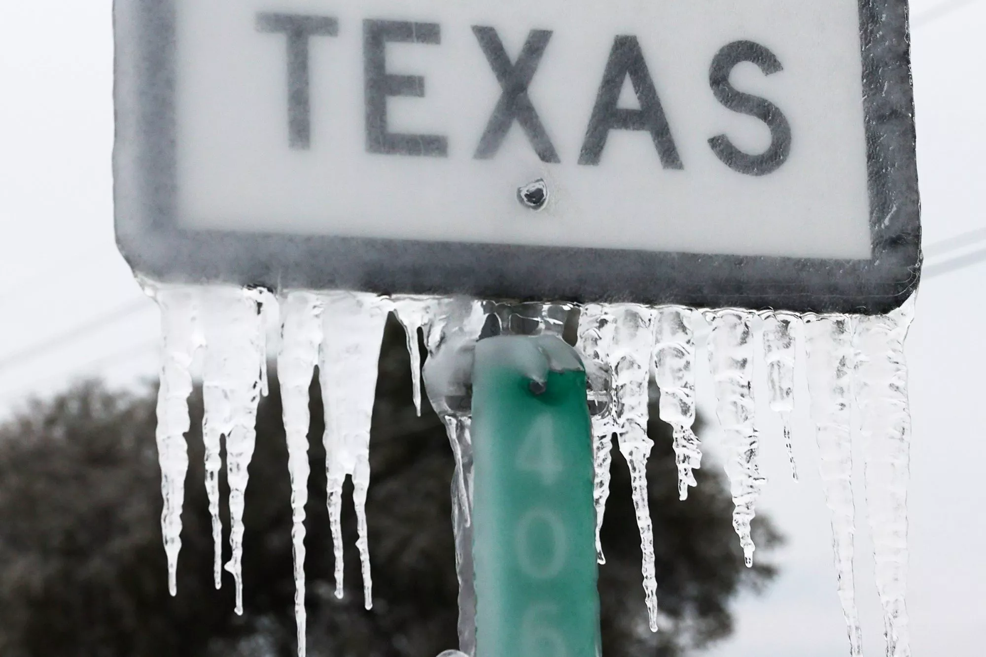
In February of 2021, Winter Storm Uri swept across Texas, bringing record-breaking cold temperatures and heavy precipitation (NOAA, 2023). The storm produced the longest stretch of freezing temperatures in the state’s history, triggering widespread power outages, burst pipes, dangerous road conditions, and numerous accidents (NOAA, 2023 and Watson P, 2021). At some point during the storm, millions of civilians (more than 2 out of 3 people) were left with no electricity or heat during the subfreezing conditions (Watson P, 2021).

This project aims to analyze the effects of the extreme weather associated with Winter Storm Uri on Houston’s power grid, and investigate the relationship of household median income as a possible co-variable to the power outage distribution.

Credits to Joe Raedle/Getty. Image obtained from the People.

Datasets

The night light raster data is Visible Infrared Imaging Radiometer Suite (VIIRS) from NASA’s Level-1 and Atmospheric Archive & Distribution System Distributed Active Archive Center (LAADS DAAC). VIIRS collects both visible and infrared imagery on 10 by 10 tiles. Houston, Texas is located between two tiles (h08v05 and h08v06). Therefore, we will need to merge the tiles together. For this project, we will be looking at night light pre (Feb 7) and post (Feb 16) the storm.
The road and house data is originally from Open Street Map but taken from a Geofabrik (a third party). Highways account for a large portion of the night lights. During Winter Storm Uri, there was most likely a reduction of traffic as roads iced over and were shutdown. To ensure highways are not classified as blackouts, we must remove highways from our night light data.
Texas’s socioeconomic data is the 2019 census track information from the U.S. Census Bureau’s American Community Survey.

Initial Steps

Always, the first step is to load all necessary libraries.

Code

# Import libraries 

library(tidyverse)
library(tmap) # for map making
library(kableExtra) # for table formatting

library(geodata) # for spatial vector data
library(stars) # for spatial vector data

library(raster) # for spatial raster data 
library(terra) # for spatial raster data

Then, load in all the datasets.

Code

# Night lights data ************************************************************
# read in with read_stars()... which is used with sf functions
light_1 <- read_stars(here::here("Posts","winter_storm_uri_TX_blackouts", "data", "VNP46A1", "VNP46A1.A2021038.h08v05.001.2021039064328.tif"))
light_2 <- read_stars(here::here("Posts","winter_storm_uri_TX_blackouts","data", "VNP46A1", "VNP46A1.A2021038.h08v06.001.2021039064329.tif"))
light_3 <- read_stars(here::here("Posts","winter_storm_uri_TX_blackouts","data", "VNP46A1", "VNP46A1.A2021047.h08v05.001.2021048091106.tif"))
light_4 <- read_stars(here::here("Posts","winter_storm_uri_TX_blackouts","data", "VNP46A1", "VNP46A1.A2021047.h08v06.001.2021048091105.tif"))

# Raster data could also be read in with rast()...which is used with terra functions
#l1 <- rast("data/VNP46A1/VNP46A1.A2021038.h08v05.001.2021039064328.tif")
#l2 <- rast("data/VNP46A1/VNP46A1.A2021038.h08v06.001.2021039064329.tif")
#l3 <- rast("data/VNP46A1/VNP46A1.A2021047.h08v05.001.2021048091106.tif")
#l4 <- rast("data/VNP46A1/VNP46A1.A2021047.h08v06.001.2021048091105.tif")


# Road Data - Isolating for just 'moterways' ***********************************
roads <- st_read(here::here("Posts","winter_storm_uri_TX_blackouts", "data", "gis_osm_roads_free_1.gpkg"), query = "SELECT * FROM gis_osm_roads_free_1 WHERE fclass='motorway'")

# House data - Isolating for homes only ****************************************
houses <- st_read(
  here::here("Posts","winter_storm_uri_TX_blackouts","data", "gis_osm_buildings_a_free_1.gpkg"),
  query = "
    SELECT *
    FROM gis_osm_buildings_a_free_1
    WHERE (type IS NULL AND name IS NULL)
       OR type IN ('residential', 'apartments', 'house', 'static_caravan', 'detached')
  ")


# Texas Socioeconomic Data *****************************************************

# Looking at the various layeres 
st_layers(here::here("Posts","winter_storm_uri_TX_blackouts", "data", "ACS_2019_5YR_TRACT_48_TEXAS.gdb"))

# Pulling out the geometry and income layers 
geom_texas <- st_read(here::here("Posts","winter_storm_uri_TX_blackouts", "data","ACS_2019_5YR_TRACT_48_TEXAS.gdb"), layer = "ACS_2019_5YR_TRACT_48_TEXAS")
income_texas <- st_read(here::here("Posts","winter_storm_uri_TX_blackouts","data", "ACS_2019_5YR_TRACT_48_TEXAS.gdb"), layer = "X19_INCOME")

Data Wrangling

Coordinate Reference Systems (CRS)

It is always important to know the geospatial datas’ coordinate reference systems (CRS). The CRS defines how the geospatial data is located and plotted. There are 2 CRS types: geographic (how the data is plotted on the 3D globe) and projected (how the data is plotted on a 2D map). It is important to use the correct CRS for your data and intended goal. Additionally, when merging or plotting geospatial data together, the datasets must be in the same CRS. Matching CRSs ensures that all spatial data layers align correctly, calculations are meaningful, and analytic results are trustworthy.

Code

# Create print message function to check crs 
crs_check <- function(crs1, crs2) {
  if (st_crs(crs1) == st_crs(crs2)) {
    print("its a match")
    return(crs2)
  } else {
    warning("Updating CRS")
    #crs1 <- st_transform(crs1, crs = 'EPSG:4326')
    return(st_transform(crs2, crs = st_crs(crs1)))
  }
}


# Check crs between roads, houses, and TX' geom
houses <- crs_check(roads, houses)

[1] "its a match"

Code

geom_texas <- crs_check(roads, geom_texas) # Changed these

Warning in crs_check(roads, geom_texas): Updating CRS

Code

geom_texas <- crs_check(houses, geom_texas) # Changed these

[1] "its a match"

Code

# Check crs between all the light dfs 
light_2 <- crs_check(light_1, light_2)

[1] "its a match"

Code

light_3 <- crs_check(light_1, light_3)

[1] "its a match"

Code

light_4 <- crs_check(light_1, light_4)

[1] "its a match"

Code

light_3 <- crs_check(light_2, light_3)

[1] "its a match"

Code

light_4 <- crs_check(light_2, light_4)

[1] "its a match"

Code

light_4 <- crs_check(light_3, light_4)

[1] "its a match"

Code

# Double check the CRS change worked 
st_crs(roads) == st_crs(geom_texas)

[1] TRUE

Code

st_crs(houses) == st_crs(geom_texas)

[1] TRUE

All coordinate reference systems match!

Creating a Blackout Mask

GOAL: Identify all areas in Houston, TX that experienced power outages. To accomplish this, we will merge the night light raster tiles, find areas that experienced blackouts, and crop the dataframe to Houston’s extents while excluding major highways.

(a) Combine the Night light Data

As stated before, the night light data is recorded on 10 by 10 tiles. Houston is split by two different tiles. Therefore, we have to merge the tiles together to create one picture of Houston, Texas.

Code

# Combine light data based on y
feb7sf <- st_mosaic(light_1, light_2)
feb16sf <- st_mosaic(light_3, light_4)

After creating a complete night light image of Feb 7 and 16, we need to make sure both days have the same extent. Extents refer to the geospatial range encompassed within the data.

# Check if extents match
print(st_bbox(feb7sf))

xmin ymin xmax ymax 
-100   20  -90   40

print(st_bbox(feb16sf))

xmin ymin xmax ymax 
-100   20  -90   40

The extents match, and we can move on!

(b) Finding Blackouts

Blackouts are when the power difference (between pre and post night light data) is greater than 200 nW cm^-2sr^-1. We can find this by using mathematics operations between tiles and logicals (greater than sign)

Code

# Finding where there are blackouts 
difference <- (feb7sf - feb16sf) > 200
  # Creates a list of boolean operators - returns TRUES for more than 200; FALSE for less than 200

(c) Mask Blackout Data

Mask means to convert and/or filter for specific data. In this case, we are masking for only areas that experienced a blackout (power difference > 200 nW cm^-2sr^-1). Anywhere that did not experience a blackout gets an NA value.

Code

# Create raster mask of the same resolution and extent  
diff_mask <- difference

# Assign NA to all locations that experienced a drop of less than 200 nW cm-2sr-1 change ("FALSE")
diff_mask[diff_mask == "FALSE" ] <- NA

(d) Vectorize the Blackout Mask

Convert the masked blackout dataframe to a vector by using an st_as_sf function. Then, check and change all the invalid geometries.

Code

# Convert from a raster to a vector with st_as_sf
diff_mask_vec <- st_as_sf(diff_mask)

# Invalid geometries 
which(!st_is_valid(diff_mask_vec)) # Tell us which specific ones are invalid 

# Fixing invalid geometries  
diff_mask_vec <- st_make_valid(diff_mask_vec)

(e) Crop the Blackout Mask to the Houston Area

By applying Houston’s city limits to st_bbox, we generated a bounding box representing the city’s spatial extent, which is then used, with st_crop, to clip the blackout mask data.

Code

# Create the Houston bounding box 
bound_box <- st_bbox(c(xmin =-96.5, xmax = -94.5, ymax = 30.5, ymin = 29), crs = st_crs(diff_mask))

# Crop difference vector with the bounding box 
diff_crop <- st_crop(diff_mask_vec, bound_box)
  # ANOTHER WAY: diff_crop <- difference_mask[bound_box, op = st_intersects]

(f) Exclude Highways from Blackout Area

As previously dicussed, highway traffic is typically seen from space and accounts for a large portion of the night lights. During Winter Storm Uri, roads were iced over and shut down, reducing traffic. Therefore, in order to ensure the reduction in traffic is not misinterpreted as a blackout, we must exclude the highways from the blackout mask.

First, use st_union to unionize all the highways to make the data more manageable. Secondly, make a 200m buffer zone around all highways with st_buffer .

Code

# Unionize road data to make it more manageable - Aggregating road data 
road_union <- st_union(roads) 

# Buffer areas within 200 m of all highways 
road_buffer <- st_buffer(road_union, dist = units::set_units(200, "m"))

To exclude the 200m road buffer from the blackout dataframe, we will use st_difference. This function finds all locations that are not in-common between the datasets.

Code

# Locating all blackouts NOT within the 200m highway buffer 
blackouts_200m_highway <- st_difference(diff_crop, road_buffer)

(f) Re-project the Cropped Blackout Dataset to EPSG:3083

Re-projecting means to change the CRS (the projection). We are changing the CRS with st_transform to EPSG:3083, which refers to the NAD83 / Texas Centric Albers Equal Area. This projection is better suited for the project’s scope and goals.

Code

# Changing the crs to NAD83 / Texas Centric Albers Equal Area
blackouts_epsg_hw_buff <- st_transform(blackouts_200m_highway, crs = 'EPSG:3083')

Plot Blackout Areas

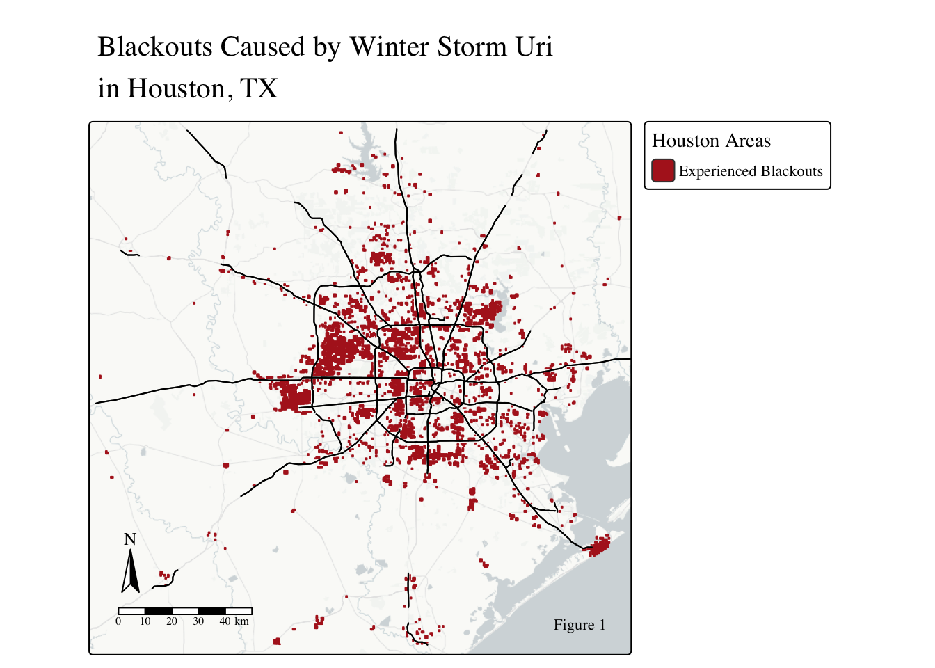
Create a map of all areas that experienced a blackout in Houston, TX during Winter Storm Uri.

Code

# Plot the backouts ! 
tm_shape(blackouts_epsg_hw_buff) + 
  tm_polygons(col = "firebrick") + 
  tm_shape(road_union) + 
  tm_lines() +
  tm_basemap("CartoDB.PositronNoLabels") +
  tm_title(text = "Blackouts Caused by Winter Storm Uri\nin Houston, TX") + 
  tm_compass(position = c("left", "bottom")) + 
  tm_scalebar(position = c("left", "bottom")) + 
  tm_credits("Figure 1", position = c("right", "bottom")) + 
  tm_layout(text.fontfamily = "Times", text.fontface = "plain") + 
  tm_add_legend(type = "polygons",
                labels = "Experienced Blackouts",
                fill = "firebrick", 
                title = "Houston Areas"
                )

Before and After Plot

GOAL: Map Houston’s night light pre (Feb 7) and post (Feb 16) the Winter Storm.

Crop Feb 7 and Feb 16 night light raster data to Houston’s extent (previously created bounding box).

Code

# Crop to Houston Texas bounding box 
feb7sf_houston <- st_crop(feb7sf, bound_box)
feb16sf_houston <- st_crop(feb16sf, bound_box)

Cloud cover can cause extreme light measurements. Therefore, to correctly plot the night light data, we need to remove all the outlier measurements by masking.

Code

# Mask to get rid of extremes 
feb7sf_houston[feb7sf_houston < 200 | feb7sf_houston > 1000] <- NA 
feb16sf_houston[feb16sf_houston < 200 | feb16sf_houston > 1000] <- NA

Plot the light intensity between Feb 7 and Feb 16 to visualize the considerable amount of blackouts from the storm.

Code

# Map feb 7 and feb 16 night light rasters 
feb7map <- tm_shape(feb7sf_houston) + 
  tm_raster(col.scale = tm_scale(values = "inferno"),
            col.legend = tm_legend(title = "Light Intensity (nW cm-2sr-1)")) +
            #title = "Light Intensity (nW cm-2sr-1)") + 
  tm_title(text = "Feb 7 Houston, TX Night Light") + 
  tm_compass(position = c("left", "bottom")) + 
  tm_basemap("CartoDB.PositronNoLabels")
  

feb16map <- tm_shape(feb16sf_houston) + 
  tm_raster(col.scale = tm_scale(values = "inferno"),
            col.legend = tm_legend(title = "Light Intensity (nW cm-2sr-1)"))+
            #title = "Light Intensity (nW cm-2sr-1)" ) + 
  tm_title(text = "Feb 16 Houston, TX Night Light") + 
  tm_scalebar(position = c("left", "bottom")) + 
  tm_credits("Figure 2") + 
  tm_basemap("CartoDB.PositronNoLabels")

tmap_arrange(feb7map, feb16map, outer.margins = 0.03)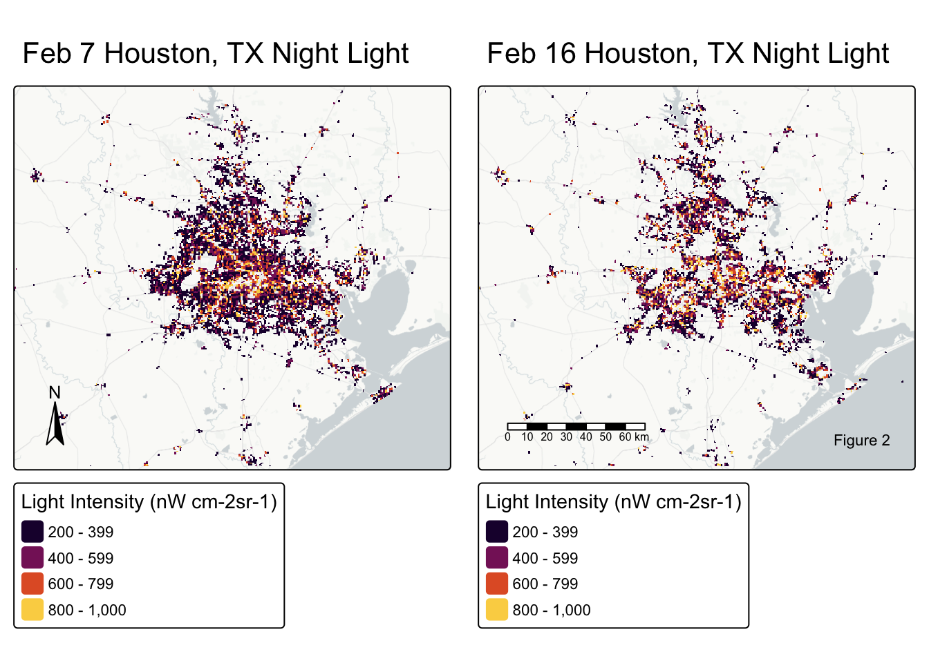

Code

# Get rid of unneccary dfs 
rm(list = c('feb7sf', 'feb16sf'))

Homes Impacted by Blackouts

GOAL: Display only homes without power during Winter Storm Uri.

First, check and transform CRSs to match. Secondly, check and fix invalid geometries.

Code

if(st_crs(houses) == st_crs(diff_crop)){ # Check if match 
  print("CRS match!")
  } else {
  warning("Updating CRS to match")
  
  # Transform to match 
  diff_crop <- st_transform(diff_crop, st_crs(houses))
  }

[1] "CRS match!"

Code

# Invalid geometries 
#which(!st_is_valid(houses))
#which(!st_is_valid(diff_crop))

# Fixing invalid geometries  
houses <- st_make_valid(houses)
diff_crop <- st_make_valid(diff_crop)

Find Homes that Experienced a Blackout

Now, we need to find the homes that experienced a blackout by introducing the Open Street Map home data. The function st_filter (with .predicate = st_intersects) will find all the houses (from Open Street Map data) that are within the blackout cropped mask.

# Homes that experienced  blackouts 
home_blackout <- st_filter(houses, diff_crop, .predicate = st_intersects)

Estimate of the Number of Homes in Houston that Lost Power

Because the home_blackout dataframe contains 1 row for every building that experienced a blackout, we can estimate the amount of homes without power by counting the number of rows with nrow.

Code

# Number of observations in the home_blackout raster 
est <- nrow(home_blackout)

# Print statement 
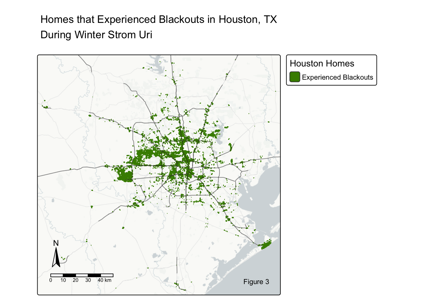
print(paste("About", est, "of Houston homes lost power"))

[1] "About 164866 of Houston homes lost power"

Map the Homes Experiencing Blackouts

Map the dataframe of homes that had a power outage.

Code

# Map it! 
tm_shape(home_blackout) + 
  tm_polygons(col = "chartreuse4") + 
  tm_basemap("CartoDB.PositronNoLabels") +
  tm_shape(road_union)+ 
  tm_lines(col = "grey20", 
           col_alpha = 0.3) +
  tm_title(text = "Homes that Experienced Blackouts in Houston, TX\nDuring Winter Strom Uri") + 
  tm_compass(position = c("left", "bottom")) + 
  tm_scalebar(position = c("left", "bottom")) + 
  tm_credits("Figure 3") + 
  tm_add_legend(type = "polygons",
                labels = "Experienced Blackouts",
                fill = "chartreuse4", 
                title = "Houston Homes"
                )

Blackouts Compared to Income

To assess whether power outages disproportionately affected certain socioeconomic groups, we integrated census-based median household income data with the blackout data. Initially, we investigated income levels between areas that experience vs did not experience a blackout to determine if income distribution differed across the two groups. This allowed us to evaluate whether lower-income communities experienced higher rates of power loss compared to more affluent areas.

Data Wrangling

(a) Join the Texas Income and Geometery Datasets

In Texas’s socioeconomic data, each row is a different census track. Whereas, the columns are different measurements for each census track. By looking at the dimensions of the two layers, we can see that the row numbers match perfectly. This makes sense because the income and geometry dataframes are just different layers of the same large dataset. Therefore, when merging the layers, we can use cbind to “stitch” the layers together, keeping all columns.

When merging datasets, its helpful to look at the dimensions before and after the merge to ensure the cbind worked properly.

Code

# Looking at dataframes 
print(paste("Dimensions of the `geom_texas` df:", nrow(geom_texas), ncol(geom_texas)))

[1] "Dimensions of the `geom_texas` df: 5265 16"

Code

print(paste("Dimensions of the `income_texas` df:",  nrow(income_texas), ncol(income_texas)))

[1] "Dimensions of the `income_texas` df: 5265 3045"

Code

# ANOTHER METHOD: dim(df) also prints the df's dimensions (made the print statement look funky) 


# Join Texas geom and incomes 
texas_df <- cbind(geom_texas, income_texas) 
# ANOTHER METHOD: LEFT JOIN: texas_df <- left_join(geom_texas, income_texas)


# Print new df's dimensions - see if the joined worked
print(paste("Dimensions of the joined df:",  nrow(texas_df), ncol(texas_df)))

[1] "Dimensions of the joined df: 5265 3061"

(b) Coordinate Reference Systems

Need to always ensure CRSs match!

Code

# Checking crs 
if(st_crs(texas_df) == st_crs(home_blackout)){ # Check if match 
  print("CRS match!")
  } else {
  warning("Updating CRS to match")
  # Transform to match 
  texas_df <- st_transform(texas_df, crs = st_crs(home_blackout))
  }

[1] "CRS match!"

(c) Filter and Merge

Filter for homes that did vs did not experience a blackout and merge the home dataset to the Texas census track data.

GOALS:

Make a datasets with homes that DID experience a blackout (home_blackout) and their median household income (texas_df) = income_bo_homes
Make a datasets with homes that did NOT experience a blackout and their median household income (texas_df) = income_NO_bo_homes

In this section, we use st_filter (with .predicate = st_intersects) to find the intersection of home_blackout and texas_df, resulting in a dataframe of homes that experienced power outages and their respective median incomes.

Code

# (1) st_filter for homes experiencing BOs
income_bo_homes <- st_filter(texas_df, home_blackout, .predicate = st_intersects) %>% 
  mutate(blackout = "TRUE") # Adding a column pertaining to experiencing a BO

Then we use st_intersections (with sparse = FALSE) and !apply to find where home_blackout and texas_df do not intersect, resulting in a dataframe of homes that did not experience a power outage and their respective median incomes.

Code

# Look for areas of intersections - Boolean Operators of TRUES (intersect) & FALSES (no intersection)
idx_intersect <- st_intersects(texas_df, home_blackout, sparse = FALSE) 

#  Looking for areas NOT included in the intersection data 
income_NO_bo_homes <- texas_df[!apply(idx_intersect, 1, any), ] %>% # Filter for all "FALSE"
  mutate(blackout = "FALSE") # Adding a column pertaining to NOT experiencing a BO

In both codes, the mutate function creates a new blackout column that states if the home does (‘TRUE’) or does not (‘FALSE’) experience a power outage.

To make sure the filtering worked, check the dimensions of each dataframe.

Code

# Look at shapes - See if filtering worked... it did! 
print(paste("Dimensions of the texas_df:", nrow(texas_df), ncol(texas_df)))

[1] "Dimensions of the texas_df: 5265 3061"

Code

print(paste("Dimensions of the home_blackout:", nrow(home_blackout), ncol(home_blackout)))

[1] "Dimensions of the home_blackout: 164866 6"

Code

print(paste("Dimensions of the income_bo_homes:", nrow(income_bo_homes), ncol(income_bo_homes)))

[1] "Dimensions of the income_bo_homes: 778 3062"

Code

print(paste("Dimensions of the income_NO_bo_homes:", nrow(income_NO_bo_homes), ncol(income_NO_bo_homes)))

[1] "Dimensions of the income_NO_bo_homes: 4487 3062"

(c) Create Dataset of all Homes in Houston

Combine the information of homes that did lose power (income_bo_homes) and homes that did not (income_NO_bo_homes). Since the columns are the same, we can use rbind to stitch together the rows.

# Merge mean income blackouts and no blackout dataframes 
income_merge <- rbind(income_NO_bo_homes, income_bo_homes)

Visualizing Blackout Experiences with Income

Mapping the median household income distributions, separating based on power outage experience.

Code

# Create my color palette 
my_palette = c('#488f30', '#a9bb5a', '#ffe896', '#ffad76', '#fc7082') 


# Map of mean (of median) income with no blackouts 
no_blackout_income_map <- tm_shape(income_NO_bo_homes) + 
  tm_polygons(fill = "B19013e1", 
              fill.legend = tm_legend(title = "Median Income ($)", 
                                      orientation = 'landscape'),
              fill.scale = tm_scale_continuous(values = my_palette)
              ) +
    tm_shape(diff_crop, is.main = TRUE) + 
  tm_title(text = "Medium Income Cenus Track for Homes with Power") +   
  tm_basemap("Esri.WorldTopoMap")


# Map of mean (of median) incomes of home that experienced blackouts 
blackout_income_map <- tm_shape(income_bo_homes) + 
  tm_polygons(fill = "B19013e1", 
              fill.legend = tm_legend(title = "Median Income ($)", 
                                      orientation = 'landscape'), 
              fill.scale = tm_scale_continuous(values = my_palette)
  ) +
  tm_shape(diff_crop, is.main = TRUE) + 
  tm_title(text = "Medium Income Cenus Track for Homes without Power") + 
  tm_scalebar(position = c('left', 'top')) + 
  tm_compass(position = c('left', 'bottom')) + 
  tm_credits(text = "Figure 5", position = c(0.7, -0.05)) + 
  tm_basemap("Esri.WorldTopoMap")

# Look at both together 
tmap_arrange(no_blackout_income_map, blackout_income_map)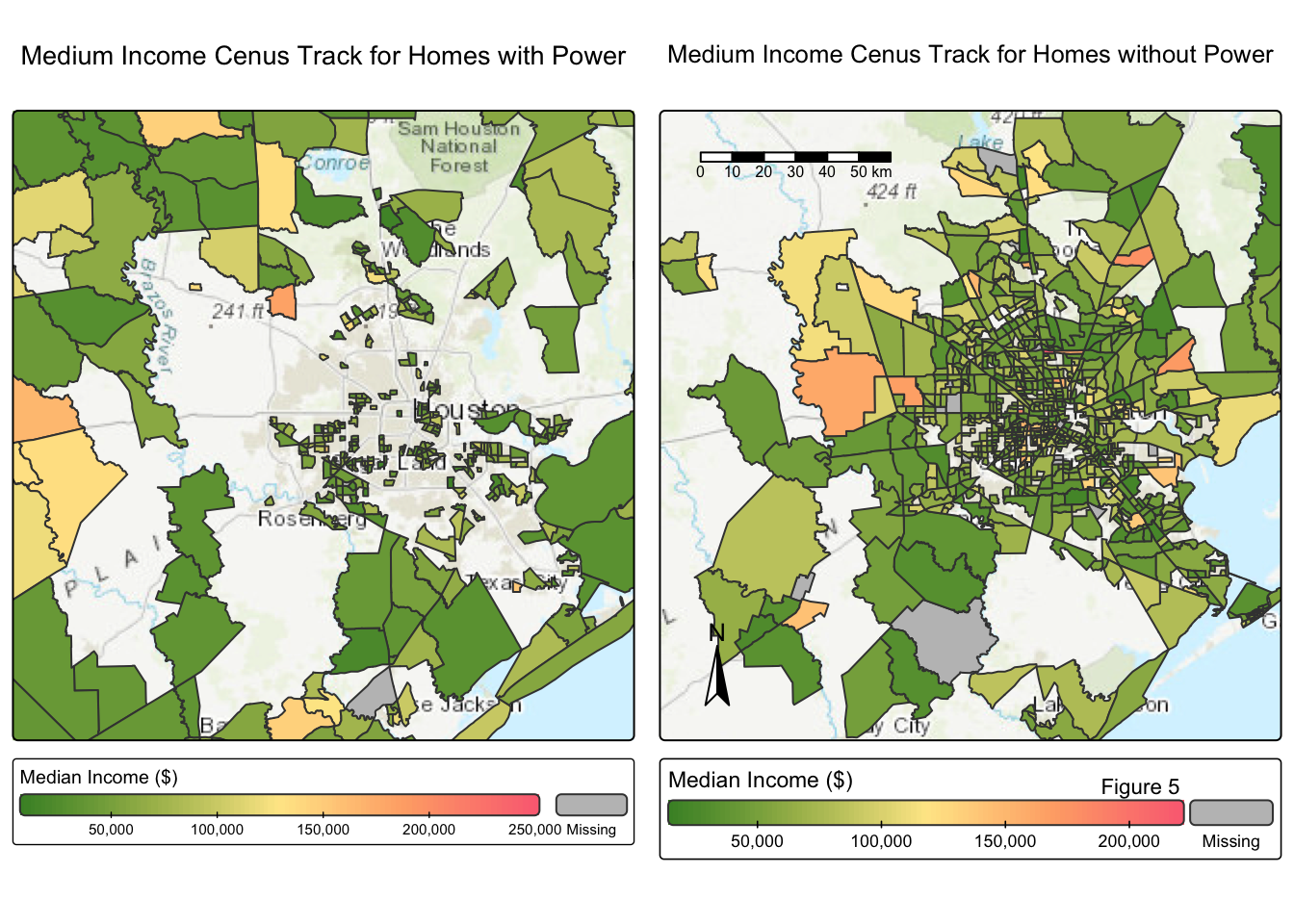

To get a better understanding of the communities that lost power, map just the income_bo_homes.

Code

# Map of households median income without power 

tm_shape(income_bo_homes) + 
  tm_polygons(fill = "B19013e1", 
              fill.legend = tm_legend(title = "Median Income that\nExperienced Blackouts ($)", 
                                      orientation = 'landscape', 
                                      position = tm_pos_out('center', 'bottom')), 
              fill.scale = tm_scale_continuous(values = my_palette)
              ) +
  tm_compass(position = tm_pos_in('left', 'bottom')) +
  tm_scalebar(position = tm_pos_in('left', 'bottom')) +
  tm_title(text = "Median Income Census Tracts in Houston, TX\nthat Experienced a Blackout During Winter Storm Uri") + 
  tm_credits("Figure 6") + 
  tm_basemap("Esri.WorldTopoMap")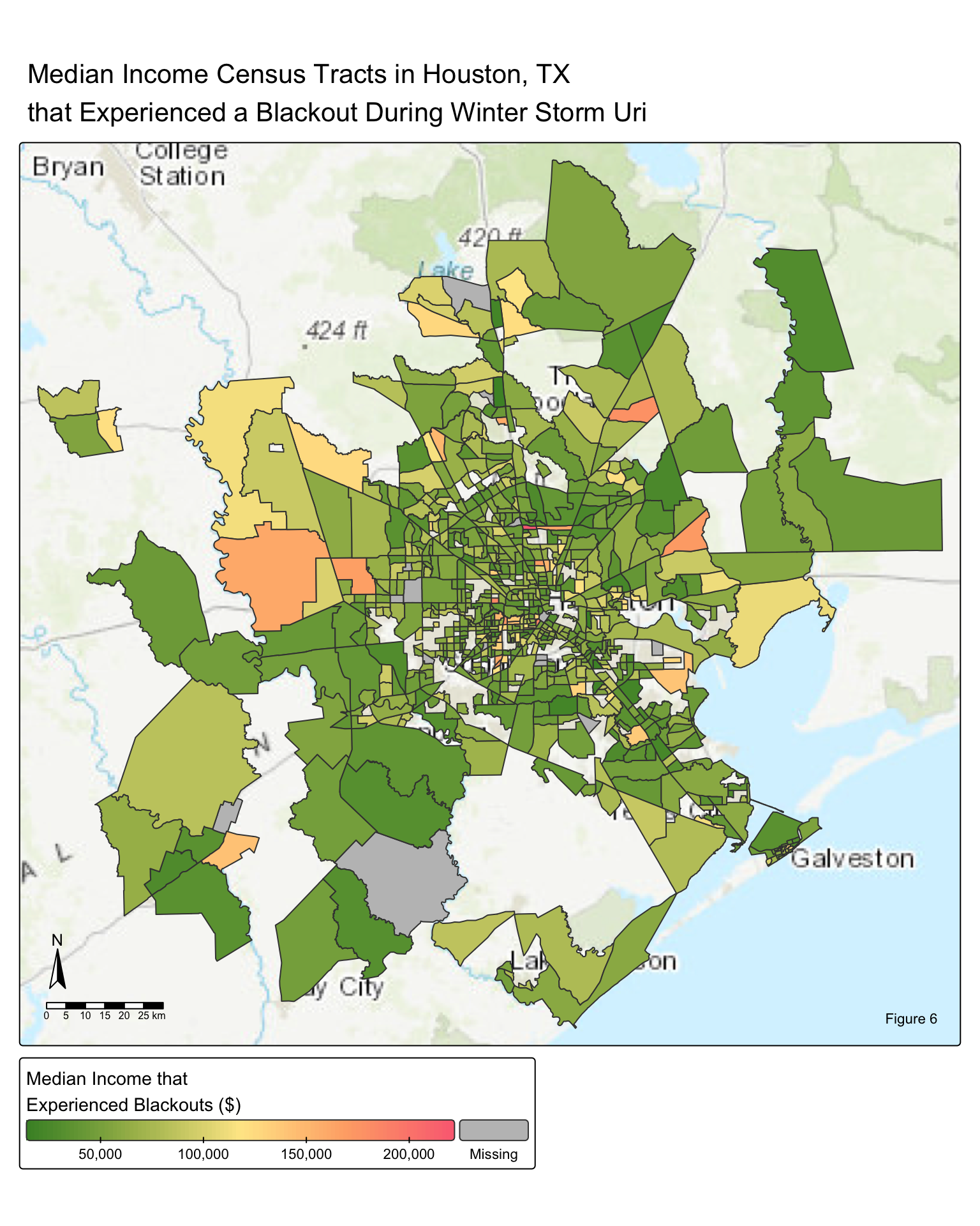

Figures 5 and 6 shows the downtown area experiencing more blackouts. However, it is difficult to understand the income distribution within the maps.

Income Classes

To better investigate if socioeconomic status (particularly income level) affected the likelihood of experiencing a blackout, we categorized the population into three income groups: low, middle, and upper class.

To do this categorization, we created a new dataframe that specified the medium income level’s class. The estimated class separation for Houston, Texas is:

Lower class: $40,000 and less
Middle class: $40,000 - $125,000
Upper class: $125,000 and above

These income class numbers are based on Fullerton, 2025.

Code

# Select only needed columns and drop geometry 
income_class <- income_merge[, c('GEOID', 'B19013e1', 'blackout')] %>% 
  st_drop_geometry() 


# Add new column based on median income for INCOME CLASSES 
income_class <- income_class %>% 
  mutate(class = case_when(
    is.na(B19013e1) ~ NA_character_, 
    B19013e1 < 40000 ~ "lower_class", 
    B19013e1 < 125000 ~ "middle_class",
    TRUE ~ "upper_class" # All others are upper class 
  ) )
# Made these income classes based on Fullerton, 2026 

# COUNTS of homes experiencing blackouts vs not per income class 
income_class_sum <- income_class %>% 
  group_by(class, blackout) %>% 
  summarise(count = n())

Plot income classes in terms of experiencing power outages or not.

Code

# Plot it 
ggplot(income_class_sum, 
       aes(x = class, 
           y = count, 
           fill = blackout)) + 
  geom_col(position="fill", # proportion plot 
           #stat = "identity",
           color = "black") + 
  scale_fill_manual(labels = c("No Blackout", "Blackout"), # labels and colors 
                    values = c("#ffad76", "#488f30")) + 
  scale_x_discrete(labels = c('Lower Class', 'Middle Class', 'Upper Class', 'NAs')) +
  labs(title = "Proportion of Households that did and did not\nExperienced Blackouts in Various Income Classes ", 
       x = "Income Classes", 
       y = "Proportion", 
       fill = "Experienced Blackout", 
       caption = "Figure 8:\nLower income class is below $40,000.\nMiddle class is $40,000 to $125,000.\n Upper class is greater than $125,000.") +
  theme_bw()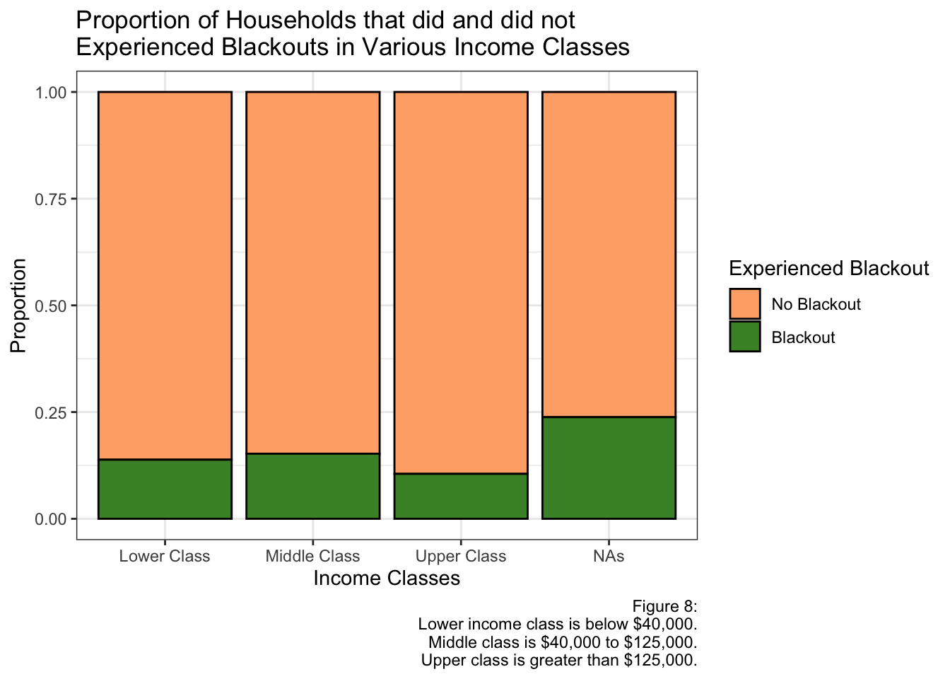

Find Percentages of Income Classes that Experienced a Blackout

To find the percentages of each income class that experiences a blackout, we will find the population within each income bracket, filter for the population that lost power in each class, then calculate the percentage (count that lost power/total count of income bracket population).

Code

# Total of homes per each income class 
class_count_total <- income_class_sum %>% 
  group_by(class) %>% 
  summarise(total = sum(count))


# Filters for home counts that experiences a blackout 
class_count_blackout <- income_class_sum %>% 
  filter(blackout == 'TRUE')

# Combine dataframes 
class_count <- left_join(class_count_blackout, class_count_total, by ='class')

# Proportions of homes that experiences a blackout per Income Class 
class_count <- class_count %>% 
  group_by(class) %>% 
  mutate(prop = 100*(count/total)) %>% 
  mutate(class = recode(class, # Change row names 
                        "lower_class" = "Lower Class", 
                        "middle_class" = "Middle Class", 
                        "upper_class" = "Upper Class", 
                        "NA" = "NA"))
  

# Creating a kable table 
knitr::kable(class_count[, c('class', 'prop')], 
                      col.names = c("Income Class", "Percentage"),
                      digits = 2, 
                      align = 'c',
                      caption = "Percentage of Each Income Class that Experienced a Blackout")

Percentage of Each Income Class that Experienced a Blackout
Income Class	Percentage
Lower Class	13.84
Middle Class	15.25
Upper Class	10.53
NA	23.81

Conclusion

In Houston, Texas, the power outage centered around the downtown area which is seen in Figures 1 - 5. Figures 6 - 8 investigate the power outages in comparison with income census blocks. The medium income distributions of homes who experienced blackouts vs did not experience blackouts are very similar and consistent with the overall medium income distribution in Houston. As shown in Figure 7 and the table, the proportion of residents experiencing blackouts is relatively consistent across income classes, ranging from about 11% to 16%. Accordingly, there is insufficient evidence to suggest that the power outages during Winter Storm Uri were biased or unjustly distributed.

Limitations: The light data was from NASA’s Level-1 and Atmosphere Archive and Distribution System Distributed Active Archive Center (LAADS DAAC) which uses Visible Infrared Imaging Radiometer Suite (VIIRS). When using satellite imagery, coarse spatial resolution and atmospheric interference can impact the study. Furthermore, the road and house data is acquired by Open Street Map which can have data completeness and accuracy issues.

Personal Statement

I am originally from Houston, Texas, and I experienced Winter Storm Uri firsthand. The storm brought unprecedented freezing temperatures to the region, overwhelming the power grid and disrupting daily life across the state. During this time, my father and I were without electricity in our home while my mother, Dr. Hessel, remained on call at the hospital for several days. It was an exceptionally difficult week with prolonged power outages, pipes bursting, hazardous conditions keeping us indoors, and widespread school closures. The event shows the importance of resilient infrastructure and highlighted how essential preparedness and coordinated response systems are during extreme weather events.

References

National Aeronautics and Space Administration (NASA). (n.d.) Level-1 and Atmospheric Archive & Distribution System Distributed Active Archive Center (LAADS DAAC). Visible Infrared Imaging Radiometer Suite (VIIRS). https://ladsweb.modaps.eosdis.nasa.gov/

OpenStreetMap. (n.d.) Planet OSM. OpenStreetMap. https://planet.openstreetmap.org/

Geofabrik GmbH. (n.d.). OpenStreetMap Data Extracts. GEOFABRIK. https://download.geofabrik.de/

United States Census Bureau. (2019). American Community Survey (ACS). United States Census Bureau. https://www.census.gov/programs-surveys/acs.

Fullerton, A. (2025). You need to make this much to be considered middle-class in Houston. FOX26. https://www.fox26houston.com/news/houston-middle-class-texas-2025

National Oceanic and Atmospheric Administration (NOAA). (2023, Feb 24). The Great Texas Freeze: February 11-20, 2021. National Centers for Environmental Information. https://www.ncei.noaa.gov/news/great-texas-freeze-february-2021

Watson, K. P., Cross, R., Jones, M. P., Buttorff, G., Granato, J., Pinto, P., … & Vallejo, A. (2021). The winter storm of 2021. Hobby School of Public Affairs, University of Houston. https://www.uh.edu/hobby/winter2021/storm.pdf

Citation

BibTeX citation:

@online{hessel2025,
  author = {Hessel, Megan},
  title = {When the {Lights} {Went} {Out:} {Mapping} {Houston’s} {Power}
    {Grid} {Collapse} {During} {Winter} {Storm} {Uri}},
  date = {2025-12-04},
  url = {https//meganhessel.github.io/Posts/analyzing_LA_fire_scars},
  langid = {en}
}

For attribution, please cite this work as:

Hessel, Megan. 2025. “When the Lights Went Out: Mapping Houston’s Power Grid Collapse During Winter Storm Uri.” December 4, 2025. https//meganhessel.github.io/Posts/analyzing_LA_fire_scars.