Global Carbon Dioxide & Methane Plume Emissions Infographic

A deep dive into global CO2 and CH4 emission sources and trends to drive climate action.

Author

Affiliation

Megan Hessel

The Bren School of Environmental Science & Management

Background

Understanding Global Carbon Dioxide & Methane Plume Emissions

Since the industrial revolution, greenhouse gas concentrations in Earth’s atmosphere have risen dramatically, fundamentally altering global climate systems (Lindsey, 2025; Casper, 2010). Carbon dioxide (CO₂) has increased from 280 parts per million (ppm) to over 410 ppm, while methane (CH₄) has risen from 700 parts per billion (ppb) to approximately 1,900 ppb (Lindsey, 2025; The Center for Biological Diversity, n.d.). These gasses absorb and re-emit infrared radiation, trapping heat within the atmosphere (process known as the greenhouse effect), driving sustained increases in global temperatures (Manabe, 2019), as illustrated in Figure 1.

The consequences of this global warming are far reaching, including rising sea levels, increased frequency of extreme weather events, and ocean acidification (Casper, 2010). Ecosystems, human health, and critical infrastructure face mounting disruption as these changes accelerate.

Emission plumes, columns of greenhouse gases and other pollutants released into the atmosphere from point sources such as industrial facilities and fossil fuel operations, are a primary driver of these concentration increases. Monitoring and quantifying these plumes is essential for understanding emission sources, informing regulatory policy, and ultimately reducing their contribution to climate change.

Figure 1. Bar plot showing global temperatures increasing from 1940 to 2025.

My Experience

Vacation for my family is water sking at Lake Fayette in Texas, which is a 2,000-4,000 acre power plant cooling lake. The Fayette Power Project burns low-sulfur coal to provide power to Austin and surrounding areas. As a kid, I would always call the smoke stacks “cloud machines” because of the visible, cloud-like gas being pumped from the top. Little did I know, the “cloud machines” were adding to air pollution and climate change. Now, as an environmental data scientist, I want to provide education and knowledge back to my communities.

Recreational water skiing on Lake Fayette with the Fayette Power Plant in the background.

The data

To reduce greenhouse gas emissions, Carbon Mapper uses remote sensing systems to track and record global plume emission data. They use ground, airborne, and satellite observational tools to find large methane and carbon dioxide emissions events, which is illustrated in Figure 2. The plumes’ source, location, gas type, and emission rate are recorded. This study will majority use the emission rate variable which is the mass of the pollutant released over a given period of time. This collection of data is made accessible to the public to promote transparency, education, and climate action.

Figure 2. Image from Carbon Mapper to explain their data collection process.

Purpose

The goal of this infographic is to further Carbon Mapper’s mission: use their public plume data to educate and “promote local climate action, globally” (Carbon Mapper). By understanding emission plumes, we can create tailored, actionable climate solutions. Solving climate change requires targeted strategies, not a “one-size-fits-all approach.” Global emissions is a complicated topic because of its interdisciplinary approach, requiring political, agricultural, and social dimensions. This infographic is the tip of the iceberg, but its futhers education and starts the conversation.

The infographic addresses these questions: 

• What are plumes made of, and what are the gasses characteristics? 

• Who is disproportionately contributing to emission plumes? 

Answering these questions will increase understanding of carbon dioxide and methane emissions and help create tailored solutions to minimize global warming.

You can check out the full data here!

The Infographic

To see the image better, right-click the image, and select “Open Image in New Tab” to open in a new tab.

Infographic of carbon dioxide and methane.

Visualizations

Plume Source Bar Plots

Carbon dioxide is emitted through human activities, mostly through burning of fossil fuels for electricity and other industrial processes. CO2 is stored in trees and soils, known as being “sequestered” within these carbon dioxide sinks. Therefore, deforestation, urbanization, and land-use change removes CO2 from these natural sinks and increases atmospheric CO2 concentration. 

Methane is commonly “leaked” from natural gas systems, such as livestock and solid waste. Livestock’s digestive processes produce and then off-gas CH4. As companies raise these animals in large quantities, CH4 emissions increase. Similarly to the digestive processes, as solid and water waste decomposes in large landfills, CH4 is off-gassed and released into the atmosphere. Industry is the most common methane source. Methane is used to produce, store, and transport oil and natural gas. Furthermore, coal mine methane (CMM) is released from mines through ventilation systems, degasification/drainage systems, and post-mining activities (such as processes, storage, and transportation) (EPA, 2026a). CCM can be captured from the ventilation and drainage systems and used for energy production (EPA, 2026a). 

Understanding the emission sources can lead to creating effective emission reduction programs. By identifying key sources for each greenhouse gas, governments and organizations can tailor policies and strategies for specific emission challenges. Some solutions for emission reduction in each sector include: 

Plume Source	Solutions
Electricity generation’s carbon dioxide emissions	Governments and organizations can set up carbon trading systems, a carbon tax, or increase funding on renewable energy sources (EPA, 2026c).
Solid waste’s methane emissions	Land-fill gas can be captured and used as a renewable energy source (EPA, 2026c).
Livestock’s methane emissions	Biogas recovery systems capture and utilize natural-by-produces from digestion for clean-burning energy fuel (Xylem, 2026; EPA, 2026c).
Oil and Gas’s methane emissions	Creating performance standards that limit methane emissions from operations and increase fuel efficiency in transportation (EPA, 2026b; EPA, 2026c).

The plot design is to resemble a smoke stack. The colors are consistent with the yellow-orange CO2 and purple CH4 colors that are used throughout the infographic. I choose the proportional bar chart to fill the smoke stacks with the sector compositions for easy comparison.

# Data Wrangling 
plumeDF_sector_tot_emission <- plumes %>% 
  group_by(ipcc_sector, gas) %>% 
  summarise(total_emissions = sum(emission_auto, na.rm = TRUE), # Total Emissions 
            .groups = "drop") %>%
  st_drop_geometry() %>% 
  filter(!ipcc_sector == "") # remove data points with no sector listed 


# Methane Sector plot 
plumeDF_CH4_sector_plot <- plumeDF_sector_tot_emission %>% 
  filter(gas == "CH4") %>% 
  ggplot() + 
  geom_bar(aes(x = "", y = total_emissions, fill = ipcc_sector), # Pie chart
           stat="identity", 
           col = "black") + 
  theme_void() + 
  labs(title = "Methane Plumes", 
       fill = "Sector") + 
  theme(plot.title = element_text(size = 13))



# CO2 Sector plot 
plumeDF_CO2_sector_plot <- plumeDF_sector_tot_emission %>% 
  filter(gas == "CO2") %>% 
  ggplot() + 
  geom_bar(aes(x = "", y = total_emissions, fill = ipcc_sector), # Pie chart
           stat="identity", 
           col = "black") + 
  theme_void() + 
  labs(title = "Carbon Dioxide Plumes", 
       fill = "Sector") + 
  theme(plot.title = element_text(size = 13), 
        legend.position = "none")
  
# Plots together 
plume_sector_plot <- (plumeDF_CO2_sector_plot | plumeDF_CH4_sector_plot) 

Proportional stacked bar plot of sector emissions for CH4 and CO2 in the shape of smoke stacks. CO2 emission are main from electricity generation, whereas CH4 emissions are from oil & gas, solid waste, and coal mining.

Greenhouse Gas Background Plots

Carbon dioxide has a much higher atmospheric concentration than methane as it is emitted through the burning of fossil fuels, deforestation, and industrial processes. Methane, on the other hand, is emitted through a larger variety of sources including solid waste, natural gas and petroleum systems, and livestock. Since pre-industrial times, both greenhouse gas emissions have increased with human activities, just at different rates and concentrations. While CO2 concentration is much greater than than CH4, methane has 27-30 times greater global warming potential (gwp) (Kathairos, 2023; EPA, 2025). This means that one CH4 molecule absorbs the same infrared radiation (heat) as 25-30 CO2 molecules over 100 years (Kathairos, 2023; EPA, 2025). In a 20 year time period, methane traps 81-83 more heat than carbon dioxide (EPA, 2025). This is important because both greenhouse gases have vastly different concentrations and global warming potentials which makes them both very important to climate change. Understanding both gasses characteristics and trends will help create effective climate action solutions. 

For plot design, I went with a simple bar chart for the atmospheric concentrations and a proportional area circle chart for the global warming potential. Both basic/traditional plots illustrate the differences in carbon dioxide and methane in a clean and straightforward way.

# gas colors 
gas_pal <- c("CH4" = "#7F28D5", 
             "CO2" = "#FFBF44")

# Total emission plot 
gas_total_emissions <- plumes %>% 
  group_by(gas) %>% 
  summarise(emission_auto = sum(emission_auto, na.rm = TRUE)) %>% 
  st_drop_geometry() %>% 
  ggplot() + 
  geom_col(aes(x = gas, y = emission_auto, fill = gas), col = "black") + 
  scale_fill_manual(values = gas_pal) +
  theme_minimal() + 
  labs(y = "Total Emission (kg/hr)") + 
  theme(axis.title.x = element_blank(), 
        legend.position = "none")



# GWP Comparison Circle chart
gwp <- data.frame(gas = c("CO2", "CH4"), 
                  life_time = c(500, 12.4), # Chem life times 
                  gwp = c(1,28)) # global warmining potential
gas_gwp_plot <- ggplot() +
  geom_point(data = gwp, 
             mapping = aes(x = gas, y = 0, size = gwp, fill = gas), 
             shape = 21, color = "black", alpha = 0.7) +
  scale_size_area(max_size = 20) +  # Ensures area ~ value
  coord_fixed(ratio = 5) +          # Keep circles round
  theme_minimal() +
  scale_fill_manual(values = gas_pal, guide = "none") + 
  labs(
    title = "Global Warming Potiential (gwp)",
    size = "Value"
  ) +
  theme(axis.text.y = element_blank(),
        axis.ticks.y = element_blank(), 
        axis.title.y = element_blank(), 
        axis.title.x = element_blank(), 
        legend.position = "none")

gas_gwp_plot / gas_total_emissions

IMAGE: Bar plot illustrating carbon dioxide emission rates are far beyond methane’s abundance, reaching over 1 billion kg/hr. The proportional area circle plot displays methane having about a 28 times larger global warming potential than CO2.

Emission Per Country Stream Plot

To understand the distribution of plume emissions on spatial and temporal scales, I created a stream plot. This plot type illustrates how carbon dioxide and methane emission rates rise and fall overtime in the top emitter countries. CO2 and CH4 are emitted at completely different rates. Having CO2 emission rates extend upwards and CH4 emission rates extend downwards allows for two different y-axis in order to compare the peaks and troughs of the greenhouse gas emission rates. 

The Arab Gulf States, including Qatar, Kuwait, Saudi Arabia, Omen, United Arab Emirates (UAE), and Bahrain, have the highest CO2 emissions per capita. These are small, oil and gas dependent nations. Fossil fuel combustion is where they get the majority of their energy and economic revenue (Ali & Abdalla, 2025). Some of these countries have recently taken strides to create climate action plans (Pasquali, 2025; Ali & Abdalla, 2025). Transitioning these energy systems toward sustainable alternatives, supported by governance reform, is important to yielding significant emission reductions and helping reduce climate change.

Furthermore, Turkmenistan has consistently been the lead methane emitter because of their deteriorating oil and gas infrastructure (IMOE & UN Environment Programme, 2025; He et al, 2024). Modernization is necessary to minimize the large CH4 emissions per capita from Turkmenistan (IMOE & UN Environment Programme, 2025).

The per-capita stream plot reveals which countries carry the heaviest emission burden relative to their population size, and where targeted climate action could have the greatest impact.

# Data wrangling 
plumes_per_country <-plumes_country %>% 
  st_drop_geometry() %>% 
  group_by(name_long, year = year(datetime), month = month(datetime), gas) %>%  # Find avg and sum for each month of each year 
  summarise(total_emissions = sum(emission_auto, na.rm = TRUE),
            avg_emissions = mean(emission_auto, na.rm = TRUE),
            pop = mean(pop),
            .groups = "drop") %>%
  mutate(year_dec = year + (month - 1) / 12, #decimal year 
         emission_total_capita = (total_emissions/pop), 
         emission_per_million = (total_emissions/pop) * 1e6) # per 1 million people


# Top 10 green house gas emitters 
top_countries_CH4 <- plumes_per_country %>%
  filter(gas == "CH4") %>%
  group_by(name_long) %>%
  summarise(total = sum(emission_per_million)) %>%
  slice_max(total, n = 10) %>%
  pull(name_long)


top_countries_CO2 <- plumes_per_country %>%
  filter(gas == "CO2") %>%
  group_by(name_long) %>%
  summarise(total = sum(emission_per_million)) %>%
  slice_max(total, n = 10) %>%
  pull(name_long)



# Plot for CH4
CH4_per_country <- plumes_per_country %>% 
  filter(gas == "CH4", 
         year >= 2023, 
         name_long %in% top_countries_CH4) %>% 
  #mutate(emission_per_million = -emission_per_million) %>% 
  ggplot(aes(x = year_dec, #  use decimal year 
             y = emission_per_million, 
             fill = name_long)) +
  geom_stream(type = "ridge",  bw = 0.85) + 
  geom_stream_label(aes(label = name_long), 
                    type = "ridge", 
                    size = 2.5) +
  labs(fill = "Countries") +
  theme_minimal() + 
  theme(axis.title.y = element_blank(), 
        axis.title.x = element_blank())


# Plot for CO2
CO2_per_country <- plumes_per_country %>% 
  filter(gas == "CO2", 
         year >= 2023, 
         name_long %in% top_countries_CO2) %>% 
  ggplot(aes(x = year_dec, #  use decimal year 
             y = emission_per_million, 
             fill = name_long)) +
  geom_stream(type = "ridge",  bw = 0.85) + 
  geom_stream_label(aes(label = name_long), 
                    type = "ridge", 
                    size = 2.5) +
  labs(fill = "Countries") +
  theme_minimal() + 
  theme(axis.title.y = element_blank(), 
        axis.title.x = element_blank())

Stream plot illustrating Qatar and Kuwait emit disproportional CO2 concentrations, and Turkmenistan dominate CH4 emissions.

Design Elements

Graphic Form

Graphic Form: I used various plot types. Each graphic form was chosen to appeal to the “common person.” The goal is to find the most minimalistic way to convey the plot’s message. Therefore, I use commonly known and recognizable plot types such are bar, circle, and stream plots

The bar and circle plots compare the proportion of CO2 and CH4 abundance and global warming potential. The proportional stack bar chart illustrates the difference between the gasses’ plume sources. Finally, the stream plot allows the ability to examine how countries’ emissions changed overtime.

Text

Text: All of my text was edited or added in Affinity. Affinity offers flexibility with captions, lables, texts, and titles. These elements can be easily changed overtime as I continually alter the infographic.

For the topography, I wanted a clean, industrial-like font as the titles and a more simple, yet professional font for the sub-text. With numbers in the axises and text boxes, the fonts being mono-spaced (which is where all numbers and letters have the same width) was important. Therefore, I decided on Krungthep font for titles and kefa font for any sub-text.

Themes

Themes: Plot themes were kept simple by including only essential information. I removed axis titles and grid lines when necessary.

Colors

Colors: The color choices are picked from Carbon Mapper’s website who supplied all data used for the infographic. The carbon dioxide and methane colors are an orange-yellow and a purple which are Carbon Mapper’s main color theme and color-blind friendly. The orange-yellow represents CO2 emission characteristics while the purple represents CH4 emission characteristic for each plot and text feature. For the sector plot, the green shades represent countries in the top ten emitters for both CO2 and CH4.

Additionally, plumes are a heavy and dark topic. Therefore, the dark background color is to portray the same gloomy feeling. 

General Design

General Design: The inforgraphic is divided into 3 parts: gas characteristics, gas sources, and country emissions overtime. As people typically read left to right, the gas characteristics are on the top left to build the story. After absorbing the introductory information, such as abundance and gwp, the story naturally flows to the plume sources and stream plots where the viewer examines the sectors and countries emission trends.

The color scheme is designed to support the overall layout. All orange-yellow plot elements and text relate to CO2 information, while purple plot elements and text represent CH4 information. This consistent use of color makes it easier to compare all three sections of the infographic.

Message

Message: Most climate conversations focus on total emissions, which typically target the Unites States, China, and India. But total emissions only tell part of the story. This inforgraphic dives deeper into per-capita and per-source emission trends to uncover where actionable climate solutions are possible.

In the stream plot, we learn Turkmenistan emits more methane per capita than any other country in the dataset. Turkmenistan oil and gas infrastructure was developed during the Soviet era in the 1900s (IMOE & UN Environment Programme, 2025; He et al, 2024). The country’s vital pipelines are deteriorating and leaking large amounts of methane into the atmosphere (IMOE & UN Environment Programme, 2025). With international investment and cooperation to help modernize its infrastructure, Turkmenistan represents one of the highest-leverage opportunities to reduce global CH4 emissions. Turkmenistan currently does have a plan to become 100% renewable energy by 2050 (Satymov, Bogdanov, & Breyer, 2021).

The Arab Gulf States include Saudi Arabia, United Arab Emirates (UAE), Qatar, Kuwait, Bahrain, and Oman. Many of these countries have the highest CO2 emissions per capita because of their heavy fossil fuel dependency and high energy consumption (Ali & Abdalla, 2025). Transitioning these energy systems toward sustainable alternatives, supported by governance reform, could yield significant emission reductions.

The goal is not to point figures. It’s to inspire targeted, cooperative action. Climate solutions are not a “one-size-fits-all.” Therefore, knowing where emissions concentrate helps us direct efforts where they matter most.

Accessibility

Accessibility: The orange-yellow and purple palette is color blind friendly, ensuring contrasts remain distinguishable. The numerous countries in the stream plot required more colors, making full colorblind compliance difficult. Nevertheless, every trend is labeled or explained in the accompanying text so the data remains accessible to all readers. Furthermore, all images and figures have alt text ensuring accessibility for visually impaired users.

DEI

Diversity, Equity, and Inclusion (DEI): Accessibility and equity were central considerations in this infographic. Color choices and text elements were made with colorblind accessibility in mind. Alt text was added to ensure a broad audience could understand the material. Beyond visual accessibility, the framing of this infographic was intentional. Climate narratives often center large, wealthy nations while overlooking the historical and economic context of smaller ones. Looking at emissions per-capita allows for understanding of countries like Turkmenistan who inherited deteriorating Soviet-era infrastructure and the Gulf states whose systems were built on fossil fuels before climate consequences were understood. This goal of the infographic is to NOT point fingers. It recognizes that equitable climate solutions require understanding each country’s unique constraints and opportunities. This study acknowledges that the countries highlighted are not historical drivers of climate changes; they are the current countries needing solutions.

# Load in libraries 
library(jpeg)
library(png)
library(tidyverse)
library(sf)
library(patchwork)
library(ggstream)

#............................load Data...........................
# Loading in Carbon Mapper  data 
# Plumes by year
plumes_2016 <- read.csv(here::here("Posts", "plume_infographic","data", "plume_yearly", "export_2016_2017", "export_2016-01-01_2017-01-01.csv")) 
plumes_2017 <- read.csv(here::here("Posts", "plume_infographic","data", "plume_yearly", "export_2017_2018", "export_2017-01-01_2018-01-01.csv")) 
plumes_2018 <- read.csv(here::here("Posts", "plume_infographic","data", "plume_yearly", "export_2018_2019", "export_2018-01-01_2019-01-01.csv")) 
plumes_2019 <- read.csv(here::here("Posts", "plume_infographic","data", "plume_yearly", "export_2019_2020", "export_2019-01-01_2020-01-01.csv")) 
plumes_2020 <- read.csv(here::here("Posts", "plume_infographic","data", "plume_yearly", "export_2020_2021", "export_2020-01-01_2021-01-01.csv")) 
plumes_2021 <- read.csv(here::here("Posts", "plume_infographic","data", "plume_yearly", "export_2021_2022", "export_2021-01-01_2022-01-01.csv")) 
plumes_2022 <- read.csv(here::here("Posts", "plume_infographic","data", "plume_yearly", "export_2022_2023", "export_2022-01-01_2023-01-01.csv")) 
plumes_2023 <- read.csv(here::here("Posts", "plume_infographic","data", "plume_yearly", "export_2023_2024", "export_2023-01-01_2024-01-01.csv")) 
plumes_2024 <- read.csv(here::here("Posts", "plume_infographic","data", "plume_yearly", "export_2024_2025", "export_2024-01-01_2025-01-01.csv")) 
plumes_2025 <- read.csv(here::here("Posts", "plume_infographic","data", "plume_yearly", "export_2025_2025", "export_2025-01-01_2025-10-01.csv")) 

# Combines the years into `plumes`
plumes <- rbind(plumes_2016, plumes_2017, plumes_2018, plumes_2019, plumes_2020, plumes_2021, plumes_2022, plumes_2023, plumes_2024, plumes_2025)

# Make plumes spatial
plumes <- st_as_sf(plumes, coords = c('plume_longitude', 'plume_latitude'), crs = 'EPSG:4326')

# Add country data 
counties <- spData::world

# JOIN Plume + Country data 
plumes_country <- st_join(counties, plumes)

# Create color palettes 
gas_pal <- c("CH4" = "#7F28D5", 
             "CO2" = "#FFBF44")

#...............................................................................
#                                                                              .
#  Sector Plot                                                                 .
#                                                                              .
#...............................................................................

#......................... Wrangle ..........................
# Find total emissions for each sector for each gas 
plumeDF_sector_tot_emission <- plumes %>% 
  group_by(ipcc_sector, gas) %>% 
  summarise(total_emissions = sum(emission_auto, na.rm = TRUE), # Total Emissions 
            .groups = "drop") %>%
  st_drop_geometry() %>% 
  filter(!ipcc_sector == "") # remove data points with no sector listed 



# Turn sectors into factors 
# plumeDF_sector_tot_emission$ipcc_sector <- factor(plumeDF_sector_tot_emission$ipcc_sector,
#                                                      levels = sector_order)

# ------------ CH4 plot ------------

# Methane Sector plot 
plumeDF_CH4_sector_plot <- plumeDF_sector_tot_emission %>% 
  filter(gas == "CH4") %>% 
  ggplot() + 
  #geom_treemap(aes(area = total_emissions, fill = ipcc_sector)) + # tree map 
  geom_bar(aes(x = "", y = total_emissions, fill = ipcc_sector), 
           stat="identity", 
           width = 0.7, 
           color = "black") + 
  #coord_polar("y", start=0) + # This makes it a pie plot 
  #scale_fill_manual(values = sector_color_pal) +
  theme_void() + 
  labs(title = "Methane Plumes", 
       fill = "Sector") + 
  theme(plot.title = element_text(size = 13))


# ------------ CO2 plot ------------

# CO2 Sector plot 
plumeDF_CO2_sector_plot <- plumeDF_sector_tot_emission %>% 
  filter(gas == "CO2") %>% 
  ggplot() + 
  #geom_treemap(aes(area = total_emissions, fill = ipcc_sector)) + # tree map 
  geom_bar(aes(x = "", y = total_emissions, fill = ipcc_sector), # Pie chart
           stat="identity", 
           width = 0.7, 
           color = "black") + 
  #coord_polar("y", start=0) + 
  #scale_fill_manual(values = sector_color_pal) +
  theme_void() + 
  labs(title = "Carbon Dioxide Plumes", 
       fill = "Sector") + 
  theme(plot.title = element_text(size = 13), 
        legend.position = "none")
  
# Plots together 
plume_sector_plot <- (plumeDF_CO2_sector_plot | plumeDF_CH4_sector_plot) +
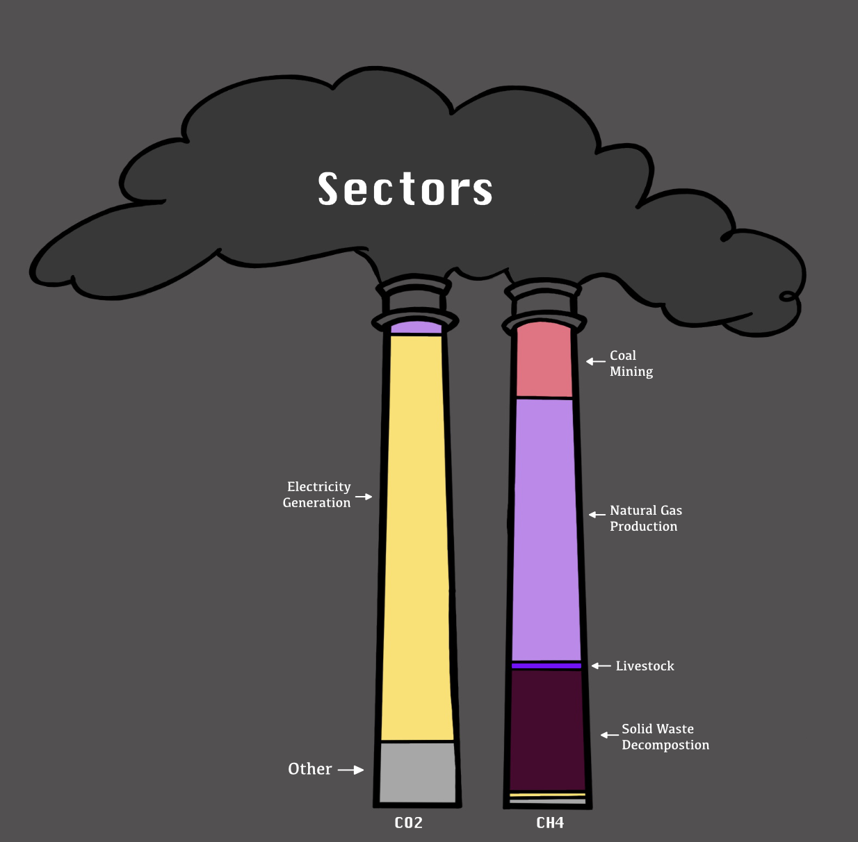
  plot_annotation(title = "Sector Composition", 
                  subtitle = "The oil and natural gas sector emits the most methane,\nwhereas Electricity Generation emits the most carbon dioxide.", 
                  caption = "Data Source: Carbon Mapper",
                  theme = theme(plot.title = element_text(size = 17, face = "bold"), 
                                plot.subtitle = element_text(size = 12, color = "gray60"),
                                plot.caption = element_text(face = "italic")))

# ggsave(filename = here::here("final_figs", "sector.pdf"), 
#        plot = plume_sector_plot, 
#        height = 7,
#        width = 9
#        )


#...............................................................................
#                                                                              .
#  Background CH4 and CO2 abundance and gwp plots                                                
#                                                                              .
#...............................................................................

#Bar plot of CO2 and CH4 emission concentrations  
gas_total_emissions <- plumes %>% 
  group_by(gas) %>% 
  summarise(emission_auto = sum(emission_auto, na.rm = TRUE)) %>% 
  st_drop_geometry() %>% 
  ggplot() + 
  geom_col(aes(x = gas, y = emission_auto, fill = gas)) + 
  scale_fill_manual(values = gas_pal) +
  theme_minimal() + 
  labs(y = "Total Emission (kg/hr)")


# ggsave(filename = here::here("final_figs", "gas_total_emissions.pdf"), 
#        plot = gas_total_emissions, 
#        width = 5, 
#        height = 5)


# Create dataframe for gwp 
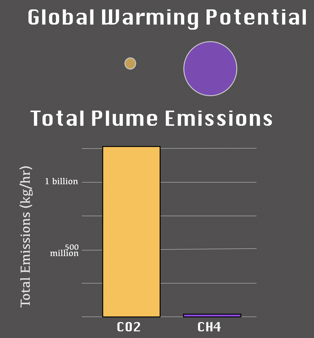
gwp <- data.frame(gas = c("CO2", "CH4"), 
                  life_time = c(500, 12.4), # Chem life times 
                  gwp = c(1,28)) # global warmining potential 

# Circle Area plots of gwp 
gas_gwp_plot <- ggplot() +
  geom_point(data = gwp, 
             mapping = aes(x = gas, y = 0, size = gwp, fill = gas), 
             shape = 21, color = "black", alpha = 0.7) +
  scale_size_area(max_size = 20) +  # Ensures area ~ value
  coord_fixed(ratio = 5) +          # Keep circles round
  theme_minimal() +
  scale_fill_manual(values = gas_pal, guide = "none") + 
  labs(
    title = "Global Warming Potiential (gwp)",
    size = "Value"
  ) +
  theme(axis.text.y = element_blank(),
        axis.ticks.y = element_blank(), 
        axis.title.y = element_blank(), 
        axis.title.x = element_blank(), 
        legend.position = "bottom")

# ggsave(filename = here::here("figs", "gas_gwp_plot.pdf"), 
#        plot = gas_gwp_plot, 
#        width = 7, 
#        height = 5)


#gas_gwp_plot / gas_total_emissions # put plots together 


#...............................................................................
#                                                                              .
#  Stream Plot                                                                 .
#                                                                              .
#...............................................................................

#......................Wrangle data ..........................

# Find each country's emissions per capita & per million people OVERTIME 
plumes_per_country_overtime <-plumes_country %>% 
  st_drop_geometry() %>% 
  group_by(name_long, year = year(datetime), month = month(datetime), gas) %>%  # Find avg and sum for each month of each year 
  summarise(total_emissions = sum(emission_auto, na.rm = TRUE),
            avg_emissions = mean(emission_auto, na.rm = TRUE),
            pop = mean(pop),
            .groups = "drop") %>%
  mutate(year_dec = year + (month - 1) / 12, #decimal year 
         emission_total_capita = (total_emissions/pop), 
         emission_per_million = (total_emissions/pop) * 1e6) # per 1 million people

# Find each country's emissions per capita & per million people in general
plumes_per_country <-plumes_country %>% 
  st_drop_geometry() %>% 
  group_by(name_long, gas) %>%  # Find total emissions per country 
  summarise(total_emissions = sum(emission_auto, na.rm = TRUE),
            avg_emissions = mean(emission_auto, na.rm = TRUE),
            pop = mean(pop),
            .groups = "drop") %>%
  mutate(emission_total_capita = (total_emissions/pop), 
         emission_per_million = (total_emissions/pop) * 1e6)

#.....................Find top 10 emitters ........................\

top_countries_CH4 <- plumes_per_country %>%
  filter(gas == "CH4") %>%
  group_by(name_long) %>%
  summarise(total = sum(emission_per_million)) %>%
  slice_max(total, n = 10) %>%
  pull(name_long)


top_countries_CO2 <- plumes_per_country %>%
  filter(gas == "CO2") %>%
  group_by(name_long) %>%
  summarise(total = sum(emission_per_million)) %>%
  slice_max(total, n = 10) %>%
  pull(name_long)

#.....................Find top 10 emitters ........................\


# ------------ CH4 plot ------------

# For CH4
plumes_CO2_per_country <- plumes_per_country_overtime %>% 
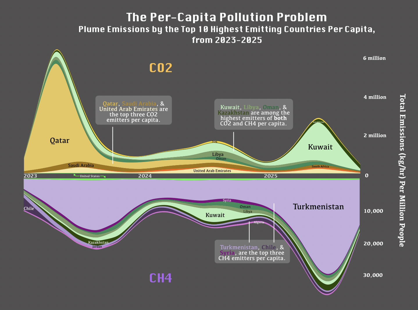
  filter(gas == "CH4", 
         year >= 2023, 
         name_long %in% top_countries_CH4) %>%  # plot just the top 10 CH4 emitters 
  ggplot(aes(x = year_dec, #  use decimal year 
             y = emission_per_million, 
             fill = name_long)) +
  geom_stream(type = "ridge",  bw = 0.85) + 
  geom_stream_label(aes(label = name_long), 
                    type = "ridge", 
                    size = 2.5) +
  theme_minimal() + 
  theme(axis.title.y = element_blank(), 
        axis.title.x = element_blank())


# ------------ CO2 plot ------------

# For CO2
plumes_CH4_per_country <- plumes_per_country_overtime %>% 
  filter(gas == "CO2", 
         year >= 2023, 
         name_long %in% top_countries_CO2) %>% # plot just the top 10 CO2 emitters 
  ggplot(aes(x = year_dec, #  use decimal year 
             y = emission_per_million, 
             fill = name_long)) +
  geom_stream(type = "ridge",  bw = 0.85) + 
  geom_stream_label(aes(label = name_long), 
                    type = "ridge", 
                    size = 2.5) +
  theme_minimal() + 
  theme(axis.title.y = element_blank(), 
        axis.title.x = element_blank())

# ggsave(filename = here::here("final_figs", "plumes_CO2_per_country.pdf"), 
#        plot = plumes_CO2_per_country, 
#        width = 6, 
#        height = 4)
# 
# 
# ggsave(filename = here::here("final_figs", "plumes_CH4_per_country.pdf"), 
#        plot = plumes_CH4_per_country, 
#        width = 6, 
#        height = 4)

References

Ali, A. H., & Abdalla, M. (2025). Energy transitions era: geopolitical characteristics and connotations in the Arab Gulf States. Sustainable Futures, 10, 100808.

Casper, J. K. (2010). Greenhouse gases: worldwide impacts. Infobase Publishing.

The Center for Biological Diversity. (n.d.) METHANE. The Center for Biological Diversity. https://www.biologicaldiversity.org/programs/climate_law_institute/global_warming_what_how_why/methane/index.html

He, T. L., Boyd, R. J., Varon, D. J., & Turner, A. J. (2024). Increased methane emissions from oil and gas following the Soviet Union’s collapse. Proceedings of the National Academy of Sciences, 121(12), e2314600121.

International Methane Emissions Observatory (IMOE) & UN Environment Programme. (2025). CURRENT STATE OF METHANE EMISSIONS IN TURKMENISTAN. https://unece.org/sites/default/files/2025-12/1.%20Current%20state%20of%20emissions%20in%20Turkmenistan.pdf

Kathairos. (2023). Methane Compared to CO₂: Why Methane Is a More Powerful Greenhouse Gas?. Kathairos Solutions Inc.https://www.kathairos.com/news/co2-vs-ch4

Lindsey, R. (2025). Climate change: atmospheric carbon dioxide. National Oceanic and Atmospheric Administration (NOAA). https://www.climate.gov/news-features/understanding-climate/climate-change-atmospheric-carbon-dioxide

Manabe, S. (2019). Role of greenhouse gas in climate change. Tellus A: Dynamic Meteorology and Oceanography, 71(1), 1620078.

Methane Imagery and Data © Carbon Mapper, https://data.carbonmapper.org

Pasquali, V. (2025). Net zero and the GCC: How the Gulf is faring on climate change. Arabian Gulf Business Insight (AGBI). https://www.agbi.com/analysis/sustainability/2025/11/net-zero-and-the-gcc-how-the-gulf-is-faring-on-climate-change/

Satymov, R., Bogdanov, D., & Breyer, C. (2021). The value of fast transitioning to a fully sustainable energy system: The case of Turkmenistan. IEEE Access, 9, 13590-13611.

United States Environmental Protection Agency (EPA). (2026a). About Coal Mine Methane. United States Environmental Protection Agency. https://www.epa.gov/cmop/about-coal-mine-methane

United States Environmental Protection Agency (EPA). (2026b). EPA’s Final Rule to Reduce Methane and Other Harmful Pollution from Oil and Natural Gas Operations and Related Actions. United States Environmental Protection Agency. https://www.epa.gov/controlling-air-pollution-oil-and-natural-gas-operations/epas-final-rule-reduce-methane-and-other

United States Environmental Protection Agency (EPA). (2026c). GHG Reduction Programs & Strategies. United States Environmental Protection Agency. https://www.epa.gov/climateleadership/ghg-reduction-programs-strategies#Supply_Chain

United States Environmental Protection Agency (EPA). (2025). Understanding Global Warming Potentials. https://www.epa.gov/ghgemissions/understanding-global-warming-potentials

Xylem. (2026). Biogas Recovery: Biogas Solutions for Methane Reduction and Resource Recovery. Xylem. https://www.xylem.com/en-us/markets/agriculture/biogas-recovery/